Part 2 in a work on my Thesis research. Here’s the Github.
I strongly recommend that if you wish to do a research project in Data Science, you begin with a data set that has some relevance to other research, but that has not been thoroughly explored. I used a data set provided by the National Center for Supercomputing Applications, which is part of the University of Illinois at Urbana-Champaign. The data came from the Blue Waters Supercomputer, funded by the National Science Foundation.
The data I used was a collection of log files, called Darshan logs, collected between February 2014 and December 2019. When I downloaded this data, it was 823.2 GB large, but this is in a very compressed format. In order to read the data, it had to be decompressed several times, then fed through a special tool that outputs a flat text file. In this fully decompressed form, the data was 296.0 TB. The largest hard drive available at the time of this writing is about 30 TB and costs about $8,000. So this data would require 10 of the largest hard drives available, and this is not feasible. I used scripts to unpack the data one file at a time, clean up the decompressed data off the disk, and aggregate the features. This way I was able to avoid running out of disk space. Even in HPC systems, ~300 TB is no trivial amount of data!
In practice, I started with a small sample of the data, and built a python script to scan the flat files for features. These feature maps of the data were then applied to each file, mapping out machine learning friendly features. The flat text files have two sections, a header and body. Each file represents one “job” in the HPC system, or one atomic execution of a scientific program that processes some information and returns a result. Some examples of counters are, POSIX number of file opens, reads, writes, bytes read/written, file system stripe width, filesystem memory offset, and histogram information about the file sizes that the job would read/write to.
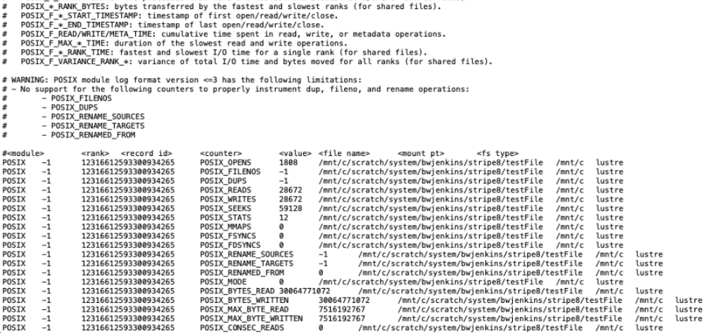
The python script that scans a Darshan file was one of the first things I had to dial in. It was built using Pandas, a popular python library that uses dataframes to process large amounts of data, in a chunked and/or distributed fashion. The chunk size was set to 109 lines per chunk. The counters are broken into key value pairs, and dataframe aggregators are used to process the entire chunk, which is then built into another dataframe, which is then itself aggregated along columns to get the final counter aggregates. Most counters are summed, however some are averaged.
The final data set, stored in CSV format with 375 MB in size, includes 875,287 jobs. The final data set is approximately six orders of magnitude smaller than the fully decompressed data set. This highlights the general scale of the data, and one of the major difficulties in this work is processing such a large volume of data. Such extreme scales highlight why this type of analysis is challenging, both within the volume of the data processed and within the values contained within said data. Asking a person to look at 900,000 histograms and draw some kind of conclusion about optimizing a network as a result of this is unlikely to product an effective result.
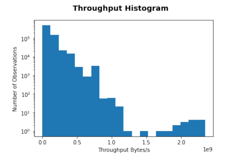
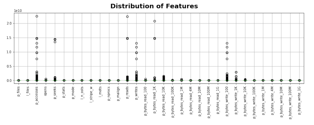
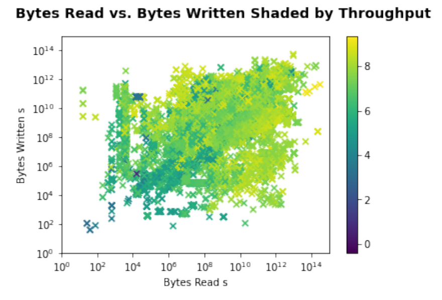
The distribution of all the dependent and independent features were skewed, multi modal and all had widely different ranges.
Now, I have explained how to process a very large data set with time and space efficient scripts, and use Python’s Pandas Data Science library to transform flat text files into aggregated features. Next time, I will describe the feature scaling techniques explored, and dive into the last steps to prepare the data for a machine learning model.